Introduction
In this use case, we showcase how, starting with a simple table containing sampling-like information (geographical coordinates and dates), it is possible to retrieve meteorological or environmental data around each of these sampling points at chosen lags before the sampling dates.
Here, let’s say that we have a dataset containing abundances of mosquitoes vectors of malaria. These mosquitoes were periodically collected in several villages of a region of Northern Côte d’Ivoire during 1.5 years. In total, 8 entomological surveys were performed in 32 villages of this area. In order to analyze the effects of temperature and rainfall on the abundance of these mosquitoes, we want to get the average temperature and cumulated rainfall for each collection point, in a 2-km radius buffer zone, one month before each collection date.
For information, the full ‘real’ dataset was published in the GBIF and exhaustively described in this data paper.
Set-up the parameters
First we load the useful packages :
library(modisfast)
library(sf)
library(terra)
library(purrr)
library(dplyr)
library(ggplot2)
library(mapview)
Then, let’s load the data and have a look at them :
head(entomological_data)
#>   mission       date village         X        Y   n
#> 1       1 2016-09-21     GUE -5.548970 9.271823 120
#> 2       1 2016-09-21     LOK -5.605484 9.186781 156
#> 3       1 2016-09-21     PEN -5.514849 9.253527  84
#> 4       1 2016-09-22     KOL -5.524137 9.288387 131
#> 5       1 2016-09-23     KAG -5.535555 9.282149 165
#> 6 1 2016-09-23 NOK -5.614132 9.251798 188- ‘mission’ is the number of the entomological survey,
- ‘date’ is the date of the survey
- ‘village’ is a 3-digit code for the village of the survey
- ‘X’ and ‘Y’ are longitude and latitude of the center of the village
- ‘n’ is the number of mosquitoes collected
The first step is to convert this dataset as an sf POINT
object :
entomological_data <- entomological_data %>%
  st_as_sf(coords = c("X", "Y"), crs = 4326) %>%
  mutate(date = as.Date(date))
Let’s map the collection points and their bounding box :
We now generate the bounding box of the collection points (ie. area
of interest) to get a POLYGON object (which is the input type for
modisfast). Then, since we will calculate the
meteorological indicators in 2-km radius buffer zones, we need to
enlarge a bit the ROI. Here, we enlarge it by 3000 m in all directions
(N, S, W, E) and we give the ROI the name “Korhogo” (the name of the
main city in the area) :
roi <- st_bbox(entomological_data)

# function expand_bbox() (Thanks @Chrisjb for the function)
source("https://raw.githubusercontent.com/Chrisjb/basemapR/master/R/expand_bbox.R")

roi <- roi %>%
  expand_bbox(.,3000,3000) %>%
  sf::st_as_sfc() %>%
  sf::st_sf()

roi$id <- "korhogo"
Next, we define the time range of interest.
Here we will first download the whole time series, and then (in step 3) filter-out the specific dates for each collection point in the next step. So for download, we set the time range as the period going from 30 days before the first collection date to the last collection date.
Download the meteorological data using modisfast
We now download the data using modisfast :
- “MOD11A2.061” = MODIS/Terra Land Surface Temperature/Emissivity 8-Day L3 Global 1 km SIN Grid v061
- “GPM_3IMERGDF.07” = GPM IMERG Final Precipitation L3 1 day 0.1 degree x 0.1 degree V07
log <- mf_login(credentials = c(Sys.getenv("earthdata_un"),Sys.getenv("earthdata_pw")))
#> Checking credentials...

urls_mod11a2 <- mf_get_url(
  collection = "MOD11A2.061",
  variables = c("LST_Day_1km","LST_Night_1km"),
  roi = roi,
  time_range = time_range )
#> Building the URLs...
#> Estimated maximum size of data to be downloaded is 2 Mb


urls_gpm <- mf_get_url(
  collection = "GPM_3IMERGDF.07",
  variables = c("precipitation"),
  roi = roi,
  time_range = time_range )
#> Building the URLs...
#> Estimated maximum size of data to be downloaded is 1 Mb


res_dl_modis <- mf_download_data(urls_mod11a2, path = "data_use_case", parallel = TRUE)
#> 1  datasets in total :  1  already downloaded and  0  datasets to download
#>
#> Actual size of downloaded data is 1 Mb
res_dl_gpm <- mf_download_data(urls_gpm, path = "data_use_case", parallel = TRUE)
#> 590  datasets in total :  590  already downloaded and  0  datasets to download
#>
#> Actual size of downloaded data is 21 Mb
And then we import it in R :
# import MODIS
modis_ts <- mf_import_data(path = dirname(res_dl_modis$destfile[1]),
                           collection = "MOD11A2.061")
#> Importing the dataset as a SpatRaster object...
# import GPM
gpm_ts <- mf_import_data(path = dirname(res_dl_gpm$destfile[1]),
                         collection = "GPM_3IMERGDF.07")
#> Importing the dataset as a SpatRaster object...

plot(modis_ts)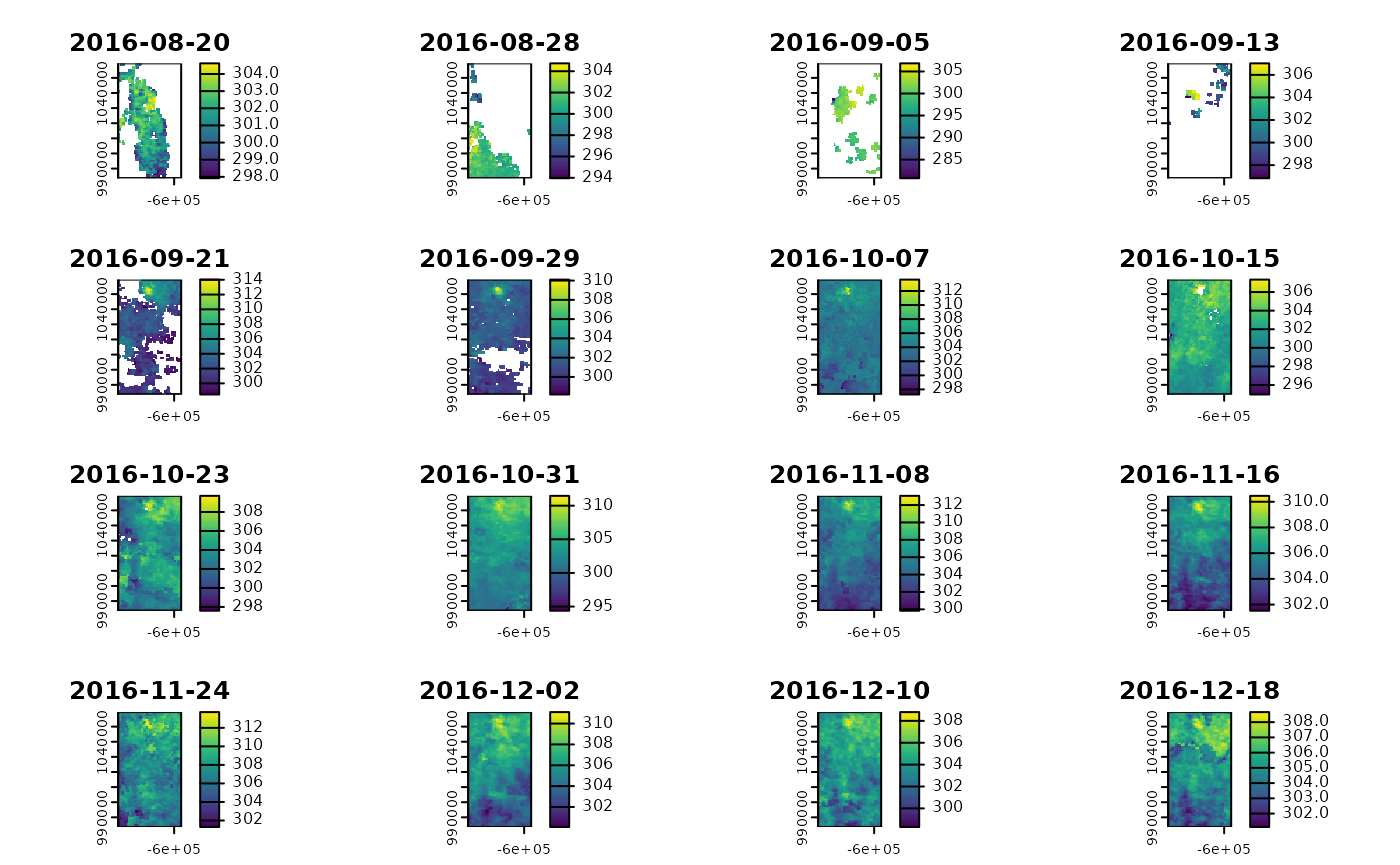
plot(gpm_ts)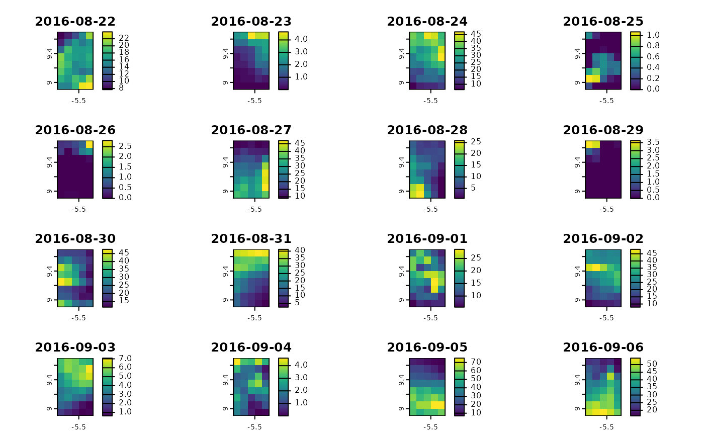
Our time series are here, let’s finish the job now !
Extract the data in 2-km radius buffer areas and 1 month before each collection date
The last step is to extract the average temperature and cumulated rainfall for each collection point in a 2-km radius buffer zone, one month before each collection date.
Below is some code for this - but feel free to adapt it, there are many ways of doing this, and the code suggested here may not be the best suited to your needs.
# generate a 2-km radius buffer area around each collection point
sp_buffer <- st_buffer(entomological_data, 2000)

# write a function that summarizes the data, given as input :
# - a buffer zone (within which the data will we summarized),
# - a SpatRaster time series,
# - a layer of interest for this SpatRaster,
# - a time range of interest
# - a function to summarize the data for the considered time frame

fun_get_zonal_stat <- function(sp_buffer, raster_ts, variable, min_date, max_date, fun_summarize){

  r_sub <- terra::subset(raster_ts, terra::time(raster_ts) >= min_date & terra::time(raster_ts) <= max_date)
  r_agg <- terra::app(r_sub[variable], fun_summarize, na.rm = T)
  val <- terra::extract(r_agg, sp_buffer, fun = mean, ID = F, touches=TRUE, na.rm = T)
  val <- as.numeric(val)

  return(val)
}

# split the dataset (needed for the execution of the function)
sp_buffer_split <- split(sp_buffer, seq(nrow(sp_buffer)))

# execute the function to get vectors
LST_1_month_bef <- purrr::map_dbl(sp_buffer_split, ~fun_get_zonal_stat(., modis_ts, "LST_Day_1km", .$date - 30, .$date, "mean"))
rain_1_month_bef <- purrr::map_dbl(sp_buffer_split, ~fun_get_zonal_stat(., gpm_ts, "precipitation", .$date - 30, .$date, "sum"))

# add columns in the original table (entomological_data) containing the extracted temperature and rainfall data
entomological_data$LST_1_month_bef <- LST_1_month_bef - 273.15  # the - 273.15  is to convert the temperature from kelvin to °C
entomological_data$rain_1_month_bef <- rain_1_month_bef

head(entomological_data)
#> Simple feature collection with 6 features and 6 fields
#> Geometry type: POINT
#> Dimension:     XY
#> Bounding box:  xmin: -5.614132 ymin: 9.186781 xmax: -5.514849 ymax: 9.288387
#> Geodetic CRS:  WGS 84
#>   mission       date village   n                   geometry LST_1_month_bef
#> 1       1 2016-09-21     GUE 120  POINT (-5.54897 9.271823)        28.87181
#> 2       1 2016-09-21     LOK 156 POINT (-5.605484 9.186781)        27.34159
#> 3       1 2016-09-21     PEN  84 POINT (-5.514849 9.253527)        28.75199
#> 4       1 2016-09-22     KOL 131 POINT (-5.524137 9.288387)        26.70374
#> 5       1 2016-09-23     KAG 165 POINT (-5.535555 9.282149)        27.98666
#> 6       1 2016-09-23     NOK 188 POINT (-5.614132 9.251798)        29.71434
#>   rain_1_month_bef
#> 1         377.1600
#> 2         366.2787
#> 3         374.3600
#> 4         362.1925
#> 5         370.0350
#> 6         368.2850
Visualize the association between the meteorological variables and the abundance of mosquitoes
We can now visualize the data :
# association between diurnal temperature and mosquito abundance
ggplot(entomological_data,aes(x=LST_1_month_bef, y=n)) + geom_point() + geom_smooth() + theme_bw() + labs(x="Average diurnal temperature\n1 month before collection", y = "Number of mosquitoes collected") 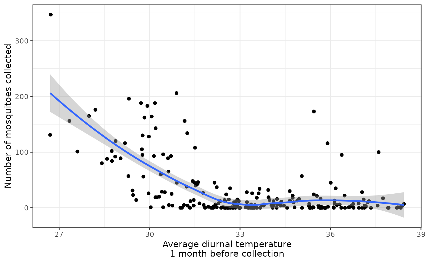
# association between rainfall and mosquito abundance
ggplot(entomological_data,aes(x=rain_1_month_bef, y=n)) + geom_point() + geom_smooth() + theme_bw() + labs(x="Cumulated rainfall\n1 month before collection", y = "Number of mosquitoes collected") 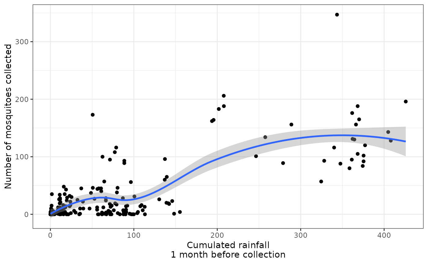
We see that overall, there is :
- a negative relationship between diurnal temperature and mosquito abundance (which makes sense : excessive temperatures might kill mosquitoes)
- a positive relationship between rainfall and mosquito abundance (which makes sense too : rainfall creates puddles, which are breeding sites)
There also seem to be non-linear relationships that could be further explored and explained.
Next steps in the analyses of the data
Next steps could imply modeling the abundances of mosquitoes using these meteorological data, for explanation or prediction purposes. To go deeper, we could also extract data from more time frames, to better apprehend several aspects of the ecology of the vectors in the study area (eg. impact of meteorological variables at the different life stages of the mosquitoes).
You may see this paper and this one for examples of full data mining works using such data.